Linear Regression
Linear Regression - Cost Function Intuition
Single Variable
Let hθ(x) be the hypothesis which predicts the value of target Y
hθ(x) = θo + θ1x
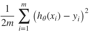
Our goal is to choose θo and θ1 such that the error between hθ(x) and the actual target Y is minimized. Intuitively, the function of Mean Square Error comes to mind.
Below is the cost function J(θ), where m is the number of training set:

Multiple Variable
Applying this to a more general problem with multi-variables:
hθ(x) = θo + θ1x1 + θ2x2 +…+ θnxn = θTx
where
- θTx is 1 by (n+1) vector
- x is (n+1) by 1 vector
- xo = 1

Gradient Decent Intuition
Gradient Decent is the method used to find θ such that the cost function J(θ) is minimized. The intuition can be understood using a simplied version of h(θ)
Assume hθ(x) = θ1x and we have following 3 data sets:
| x | y |
|---|---|
| 9 | 50 |
| 0 | -10 |
| -10 | -34 |
J(θ) = 
Example, if we let θ1 = 2,
J(θ1) = [ (9 * θ1 - 50)2 + (0 * θ1 - (-10))2 + ((-10) * θ1 - (-34))2 ] / 6 = 220
Below is the visualization of θ and J(θ), when θ is from [0, 7.8] with 0.2 increament:

Such graph indicates that the cost function is a convex function which means it’s a single bowl shape with global minimum. This is a nice feature which means no matter where we initialize the values of parameters θ, gradient decent with appropriate learning rate (α) will always converge and reach the global minimu.
Gradient Decent Algorithm
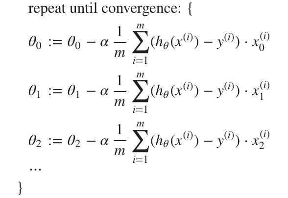
Reference taken from Andrew Ng’s ML Course on Coursera Here is the formal equation of Gradient Decent, using Batch Gradient Decent

Key points:
- x(i) is the ith row from the training set
- xj is jth feature (column), and x0 is 1
- α is the learning rate, how big each step is
about α
If α is too small, gradient decent takes long time and many iterations to converge. If α is too big, gradient decent will overshoot the global minimum and fail to converge. To know if α is good, typically one could plot J(θ) as function of number of iteration. The value of J(θ) should decrease quickly and evetually flattern
Normal Equation
Instead of taking many iterations, normal equation is able to solve the value of θT in a single step. θ = (XTX)-1XTy
- X-1 is the inverse of matrix X
- y is the target
Gradient Decent vs Normal Equation
Normal Equation does not require any iteration, nor does it require one to choose the learning rate α
However, the cost of the Normal Equation is O(n3) where n is the number of features, while gradient decent is O(kn2)Thus, when data set has huge number of features, eg 10000, it’s too costly to solve by normalization function. Instead, gradient decent would still be able to solve in reasonable amount of time.
Factors that speed-up G.D!
gradient decent works best when all feature are in the same range:
- between [-1, 1] or,
- between [-0.5, 0.5]
Two techniques can be used:
- feature scaling:
- mean normalization

Where μi is the average si is the range or standard deviation