Decision Tree
What is Decision Tree
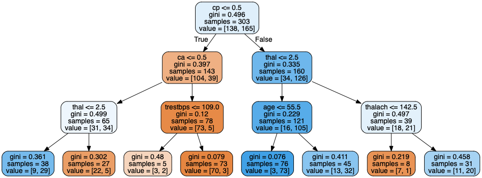
Decision Tree is like a flow chart, at the top the tree there is a ROOT, where things start. At the bottom there are leaves. Below is a visualization of a Decision Tree.

Gini impurity
The Gini impurity score tells how well the criteria splits the instances.
- Gi = 0.49 means it does not separate the training instances very well
- Gi = 0.0 means it separates the training instances perfectly

How Decision Tree works?
- calculate gini impurity for each feature, using all the records availabe
- select feature with lowest gini impurity as the root
- repeat step 1-2 for each node until
- no more records
- further seperation increases gini score
- stop criteria met
Data preparation
- Feature Scaling: Because Decision Tree looks at individual feature at a time, there is generally no need for feature scaling
- Feature Imputation
- categorical: pick majority, predict using another high correlation column
- numerical: mean or medium
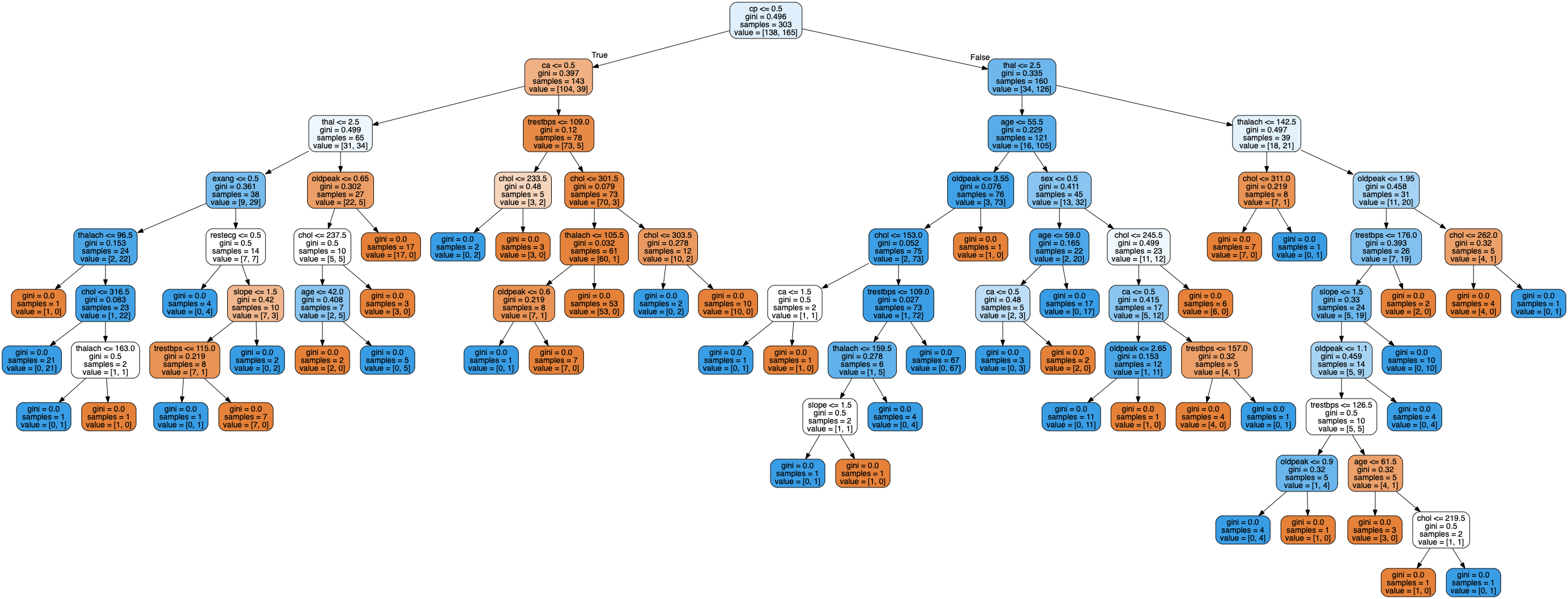
Overfitting issue in DT
Below is a decision tree build with no restriction. Clearly the second tree is having an over fitting problem.

A few way to overcome this:
- min sample leaves
- max depth: how deep the decision tree will be
Code Example
# training decision tree
from sklearn.tree import DecisionTreeClassifier
tree_clf = DecisionTreeClassifier(max_depth=5, min_samples_leaf=2)
tree_clf.fit(x_train, y_train)
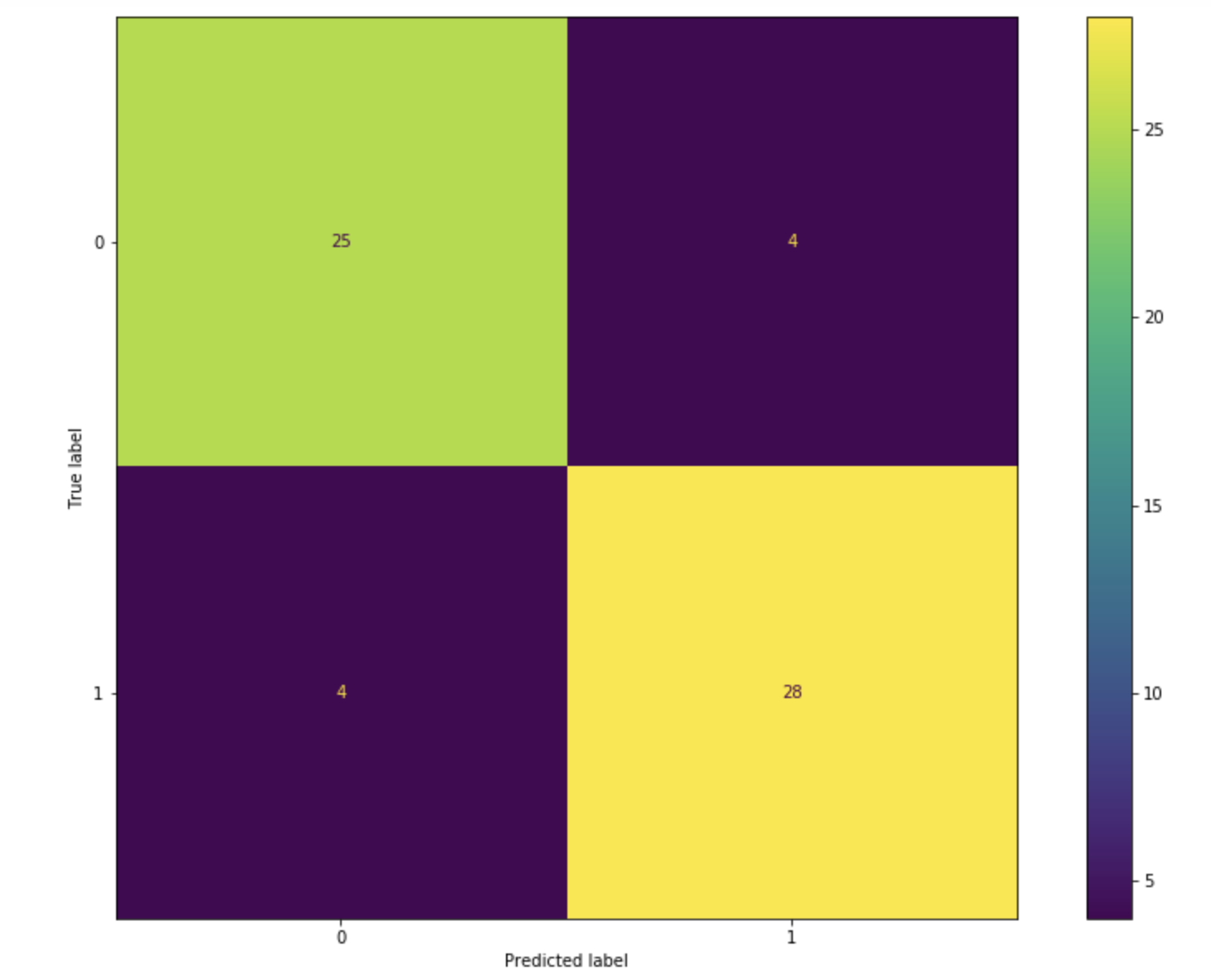
# confusion metrix
from sklearn.metrics import confusion_matrix
from sklearn.metrics import plot_confusion_matrix
fig, ax=plt.subplots(figsize=(15,10))
plot_confusion_matrix(tree_clf_3d, x_test, y_test, ax=ax)

# other score
from sklearn.metrics import confusion_matrix
from sklearn.metrics import plot_confusion_matrix
fig, ax=plt.subplots(figsize=(15,10))
plot_confusion_matrix(tree_clf_3d, x_test, y_test, ax=ax)

# output
#               precision    recall  f1-score   support
#
#            0       0.81      0.90      0.85        29
#            1       0.90      0.81      0.85        32
#
#     accuracy                           0.85        61
#    macro avg       0.85      0.85      0.85        61
# weighted avg       0.86      0.85      0.85        61
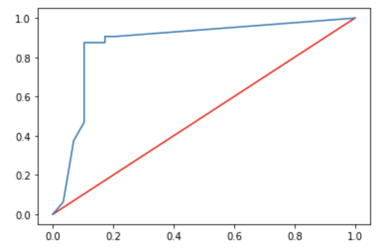
# roc curve
from sklearn.metrics import roc_auc_score, roc_curve
roc_score=roc_auc_score(y_test, y_pred)
fpr,tpr,thresholds = roc_curve(y_test, tree_clf_3d.predict_proba(x_test)[:,1])
plt.plot([0,1], [0,1], "red")
plt.plot(fpr, tpr)

RandomForest
A subset of features and a subset of samples are selected to build a bunch of shorter and simpler trees.
Collectively, they predict the result and the majority vote will be selected.
Regarding sampling for each tree, there are 2 main approaches:
- BAGGING: short for boostrap aggregation, which is sampling with replacement, allowing each record to be sampled multiple times for every predictor (aka tree)
- PASTING: sampling without replacement.
Code Example
# random forest
from sklearn.ensemble import RandomForestClassifier
rnd_clf = RandomForestClassifier()
rnd_clf.fit(x_train, y_train)
y_pred = rnd_clf.predict(x_test)

# bagging classifier
from sklearn.ensemble import BaggingClassifier
bag_clf = BaggingClassifier( DecisionTreeClassifier(), n_estimators=500, max_samples=100, bootstrap=True, n_jobs=-1)
bag_clf.fit(x_train, y_train)
y_pred = bag_clf.predict(x_test)